| 8.1 Create 2D Mask (download) |
|
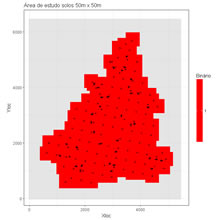
Create a 2D grid mask from sample data and a maximum distance.
Variables to customize:
varcolXY<- c(1,2) # columns of the coordinates in the GTD data frame
distanciaXY <- c(200,200) # maximum distance os a samples in X and Y directions to select the cells maskshape <- "rectangle"  # Shape for selection ellipse or rectangle xmincenter <- 25 # X coordinate of the left bottom cell centerymincenter <- 25 # Y coordinate of the left bottom cell centerncellsx <- 55 # number of cells in X directionncellsy <- 65 # number of cells in Y directioncellsizex <- 100 # cell size in X directioncellsizey <- 100 # cell size in Y direction
cellvalue <- 1 #value to assign to the selected cells nodata <- -9  #value to assign to the selected cells outside maskcolour <- c(rgb(1,0,0,0.25),rgb(.8,.8,.8,0.5)) #colours within mask and outsidemaintitle <- "Área de estudo solos 50m x 50m" # title of the graphicfileMaskGrid <- "C:/temp/Mask.OUT" # pathname and filename of a file to store the mask grid numbers. Values are writted by Y and then by X
|
 |
|
| 8.2 Estimation using the inverse of power distance (download) |
|
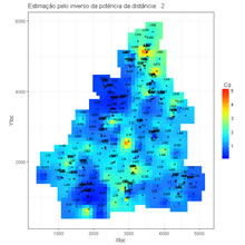
Estimation of a grid mesh by using the estimator inverse of power distance.
Variables to customize:
varcolXY <- c(1,2) # columns of the coordinates in the GTD data frame
varlistindex <- 5 # column of the variable in the GTD data frame to estimate
xmincenter <- 25 # X coordinate of the left bottom cell center
ymincenter <- 25 # Y coordinate of the left bottom cell centerncellsx <- 55 # number of cells in X direction
ncellsy <- 65 # number of cells in Y direction
cellsizex <- 100 # cell size in X direction
cellsizey <- 100 # cell size in Y direction
nodata <- -9 #value to assign to non estimated locations
power <- 2 # power value to assign to the distance
maxsamples <- 8 # maximum number of samples to use
maintitle <- paste("Estimação pelo inverso da potência da distância: ",power) # title of the image
fileMaskGrid <- "C:/temp/Mask.OUT" # file with mask values
fileOutGrid <- "C:/temp/Cd_IPD.out" # output file with the estimated results. The structure is the same of the mask file |
 |
|
| 8.3 Cross validation test for inverse power distance estimator (download) |
|
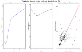
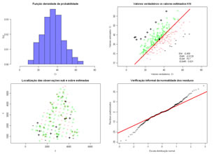
Cross validation test for estimation using the inverse of power distance, powers can range between a minimim and a maximum value, error and squared error are computed for each power and represented graphically, and the best power can be evaluated.
Variables to customize:
varcolXY <- c(1,2) # columns of the coordinates in the GTD data frame
varlistindex <- 5 # index of the GTD frame quantitative variable to test for estimation
minpower <- 0 # minimum power applied to distance to evaluate
maxpower <- 4 # minimum power applied to distance to evaluate
intpower <- 0.1 # increment of the power value to evaluate
maxsamples <- 20 # maximum number of samples to use in each estimation
escolhabi <- 12 # index of the estimation to plot a scattergram between true values and estimated values (graphic on the right)
titleGRAPH <- "Avaliação do estimador potência da distância" # title of the graphic |
 |
|
| 8.4 Ordinary and Simple Kriging demo of results (download) |
|
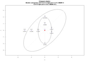
Demo of ordinary and simple kriging, inititate a simple configuration of samples and perform kriging of an unknown location to evaluate kriging weights, and estimated value.
Variables to customize:
ktype <- "KS" # KN (ordinary kriging) or KS (simples kriging)titleXY <- c("X","Y") # title of the axis X and Y
xloc <- c(-3,-2,-1,0,0,0,1.0,1.0) # X coordinates of the samples
yloc <- c(0,0,0,1,2,-2,0.3,-0.3) # Y coordinates of the samples
valor <- c(12.5,10.2,12.4,9.5,12,11,12,13) # list of hypothetical true values
xnode <- 0 # X coordinate of the location to estimate
ynode <- 0 # Y coordinate of the location to estimate
medialocal <- mean(valor) # local mean for simple kriging, can be a value or the mean of the true data
#
#  Variogram models. Models are inputed by proportion of variance (sum of Nugget effect + Sills = 1)
#
nugget_effect <- 1 # nugget effect value
nstructures <- 0 # number of structures (0, 1 or 2)
model_type <- c("Sph","Sph") # model type for each structure, can be Sph, Exp, Gauss, or Power
sill <- c(0.1,1.0) # sill of each model
range <- c(2,6.0) # range of each model
anisotropy <- c(1,1) # anisotropy factor, 1 or higher
maindir <- c(0.0,0.0) # in anisotropic, write the azimuth angle of the main direction clockwise, N direction is zero reference |
 |
|
| 8.5 kriging cross validation test (download) |
|
Cross validation test by using Simple Kriging or Ordinary Kriging. Values are estimated in the samples locations, and errors (simple and squared) are computed. Two graphics show estimation errors, first a scatterplot of true values vs estimated values and then underestimated and overestimated locations are displayed.
Variables to customize:
ktype <- "KN" # KN (ordinary kriging) or KS (simples kriging)
varcolXY <- c(1,2) # columns of the X and Y coordinated in GTD data frame
varlistindex <- 7 # column of the variable to estimate in GTD data frame
maxpercent <- 50 # percentage of mean for classification of high deviation (values in black)
nclasses <- 10 # number of classes of the histogram
nodata <- -9 # value for unestimated locations
maxsamples <- 10 # maximum number of closest samples to use in the estimation
medialocal <- mean(gtd[,varlistindex]) # global mean for simples kriging estimation, can be the average of the variable or other value
fileOutTVC="C:/temp/Cd_TVC.OUT" # output file results
#
#  Models are inputed by proportion of variance (sum of Nugget effect + Sills = 1)
#
nugget_effect <- 0.0 # nugget effect value
nstructures <- 1 # number of structures (0, 1 or 2)
model_type <- c("Sph","Sph") # model type for each structure, can be Sph, Exp, Gauss, or Power
sill <- c(1.0,1.0) # sill of each model
range <- c(1600,1) # range of each model
anisotropy <- c(2,1) # anisotropy factor, 1 or higher
maindir <- c(60.0,0.0) # in anisotropic, write the azimuth angle of the main direction clockwise, N direction is zero reference |
 |
|
| 8.6 Grid estimation by using simple or ordinary kriging (download) |
|
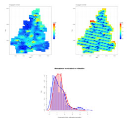
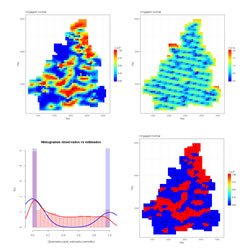
Estimation of a mesh of locations by using Simple Kriging or Ordinary Kriging. Three graphics show estimation results, the first is the estimated map of values, the second is the kriging variance map and the third displays two histograms, one of the sample data and another of the estimated values.
Variables to customize:
ktype <- "KN"  # KN (ordinary kriging) or KS (simples kriging)varcolXY <- c(1,2) # columns of the X and Y coordinated in GTD data frame
varlistindex <- 5 # column of the variable to estimate in GTD data frame
nclasses <- 20 # number of classes of the histogram
linedensity <- TRUE # add line of density in the histograms
xmincenter <- 25 # X coordinate of the left bottom cell center
ymincenter <- 25 # Y coordinate of the left bottom cell center
ncellsx <- 55 # number of cells in X direction
ncellsy <- 65 # number of cells in Y direction
cellsizex <- 100 # cell size in X direction
cellsizey <- 100 # cell size in Y direction
threshold <- -9  # Cut off value to binarize the variable and perform kriging of an indicator variable
fileMaskGrid <- "C:/temp/Mask.out" # file with mask values
fileOutGrid <- "C:/temp/Cd_KN.OUT" # output file with the estimated results. The structure is the same of the mask file^
nodata <- -9 # value for unestimated locations
maxsamples <- 8 # maximum number of closest samples to use in the estimation
medialocal <- mean(gtd[,varlistindex]) # global mean for simples kriging estimation, can be the average of the variable or other value
viewLabels <- FALSE # View true values (TRUE) or not (FALSE)
#
#  Models are inputed by proportion of variance (sum of Nugget effect + Sills = 1)
#
nugget_effect <- 0.0 # nugget effect value
nstructures <- 1 # number of structures (0, 1 or 2)
model_type <- c("Sph","Sph") # model type for each structure, can be Sph, Exp, Gauss, or Power
sill <- c(1.0,1.0) # sill of each model
range <- c(1600,1) # range of each model
anisotropy <- c(2,1) # anisotropy factor, 1 or higher
maindir <- c(60.0,0.0) # in anisotropic, write the azimuth angle of the main direction clockwise, N direction is zero reference |
|
|
| 8.7 View 2D grids and sample data (download) |
|
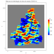
Visualization of previously estimated images by inverse of power distance or kriging.
Variables to customize:
varcolXY <- c(1,2)  # columns of the X and Y coordinated in GTD data frametitleXY <- c("X","Y") # title of X and Y axis
varlistindex <- 7 # column of the variable to estimate in GTD data frame
xmincenter <- 25 # X coordinate of the left bottom cell center
ymincenter <- 25 # Y coordinate of the left bottom cell center
ncellsx <- 55 # number of cells in X direction
ncellsy <- 65 # number of cells in Y direction
cellsizex <- 100 # cell size in X direction
cellsizey <- 100 # cell size in Y direction
nodata <- -9 # value for unestimated locations
fileNameGrid <- "C:/temp/Cd_KN.OUT" # name of the file to import and view
maintitle <- "Máscara de delimitação de área de estudo (50x50 m)" # Title of the 2D graphical display |
 |
|