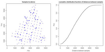
Compute distances between all pairs of samples and plot distances in a cumulative histogram.

Variables to customize: 

varcolXY <- c(1,2) # index of the GTD frame X and Y coordinatessizePOINTS <- 1  # size of the sample symbols of the left plot
titleGRAPH <- "Samples locations" # global title of the left plot

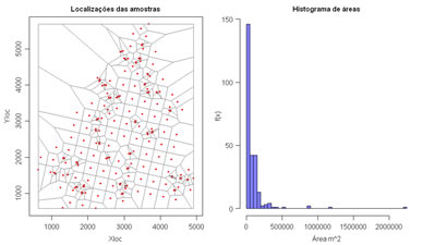
Compute Voronoi polygons and compute declustered basic statistics. An histogram of the Voronoi polygon areas are displayed at right.

Variables to customize:

varcolXY <- c(1,2) # index of the GTD frame X and Y coordinates
varlistindex <- c(5,6,7,8,9,10,11) # index of the GTD frame Qualitative Variables to recompute declustered basic statistics
titleGRAPH <- "Representação em planta das amostras de solos" # global title of the left plot
ndecimals <- 3 # number of decimal places

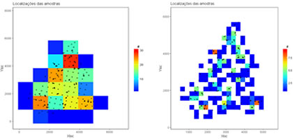
Overlap a set of samples with a mesh of cells and compute average values of several variables within each cell. After, compute global declustered basic statistics.

Variables to customize:

varcolXY <- c(1,2) # index of the GTD frame X and Y coordinates
varlistindex <- c(5,6,7,8,9,10,11) # index of the GTD frame Qualitative Variables to recompute declustered basic statistics
titleGRAPH <- "Localizações das amostras" # global title of the left plot
ndecimals <- 3 # number of decimal places
cellsizex <- 250 # size of the cells in X direction
cellsizey <- 250 # size of the cells in Y direction

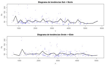
Perform a trend analysis of a quantitative variable along X and Y directions.

Variables to customize:

varcolXY <- c(1,2) # index of the GTD frame X and Y coordinatesvarlistindex <- 10 # index of the GTD quantitative variable to trend analysis
ndecimals <- 3 # number of decimal places
cellsizex <- 150 # size of the cells in X direction
cellsizey <- 150 # size of the cells in Y direction
sizePOINTS <- 2 # size of the symbols to plot