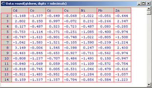
Apply a standardization formula for a set of quantitative variables. Three types of standardization can be donne:
(1)(x-m)/sd  (mean zero and standard deviation equal to one)
(2) (x-min)/(max-min) (interval [0; 1]) 
(3) 2((x-min)/(max-min))-1 (interval [-1; 1])

Variables to customize:

varlistindex <- c(5,6,7,8,9,10,11) # list of variables of GTD frame to standardizetipo <- 1 # standardization type (1), (2) or (3)ndecimals <- 3 # number of decimals

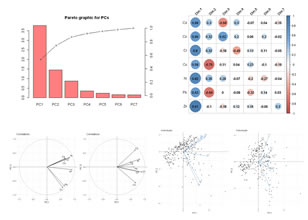
Execute a PCA for a set of quantitative variables. Four graphics are displayed as results: (1) eigenvalues histogram; (2) graphic of correlations between the quantitative variables and the Principal Components; (3) another graphic of correlations between the quantitative variables and pairs of Principal Components; (4) projection of the individuals in the Principal Components.

Variables to customize: 

varlistindex <- c(5,6,7,8,9,10,11) # index of the GTD frame Qualitative Variables to execute PCA
maxPCA <- 3 # max principal componentes to display graphics
labelSIZE <- 3 # Size of the labels within graphics
pointlabelsVIEW <- FALSE # view or not the individual labels 
viewgroups <- TRUE # display groups by ellipses in the individuals plots if already obtained by any other classification (hierarchical ou k-means)
ellipsePERCENT <- 0.5 # percentage of data to include inside each ellipse, can range between 0 and 1

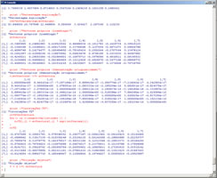
Execute a PCA step-by-step for a set of quantitative variables, in a way that all details and matrices can be followed and listed.

Variables to customize: 

varlistindex <- c(5,6,7,8,9,10,11) # index of the GTD frame Qualitative Variables to execute PCA
maxPCA <- 3 # max principal componentes to display graphics

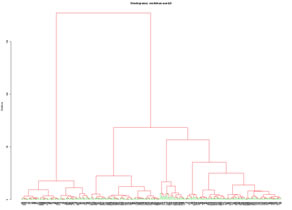
Perform a hierarchical clustering of a set of quantitative variables. Distance type and aglomeration mode should be selected. A specific number of groups can be created and conditional basic statistica for each group are diaplayed. Created groups can be seen on PCA representations.

Variables to customize: 

varlistindex <- c(5,6,7,8,9,10,11) # index of the GTD quantitative variables to execute a Hierarchical Clustering
ngroups <- 3# number of groups to generate (after that they can be plotted in PCA)
dissimilarity_method <- "euclidean"(diantance tool: euclidean, maximum, manhattan, canberra, binary, minkowski, pearson or spearman
clustering_method <- "ward.D" (compute distances between groups: ward.D, single, complete, average, centroid)

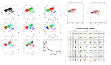
Clustering sets of individuals by using the K-means algorithm. This algorithm can run in two modes: (1) evaluation mode, trial for creation of several groups and evaluation of results; (2) separate the data into a number of previously defined groups. For (2) classification can be made with original data or the two first Principal Components. Created groups can be seen on PCA repreentations.

Variables to customize:

varlistindex <- c(5,6,7,8,9,10,11) # index of the GTD quantitative variables to execute a K-means
standardize <- FALSE # standardize all variables to mean zero and standard deviation equal to one
evaluation <- TRUE # K-means evaluation of several groups (TRUE or FALSE)
dataPCA <- TRUE # Use PC1 and PC2 to clustering data (TRUE) or use all original data (FALSE)
ngroups <- 3 # number of groups to create in non evaluation model
maxgroupsteste <- 20 #maximum number of groups to evaluate in evaluation mode
ndecimals <- 3 # number of decimals