
4. Bivariate data analysis
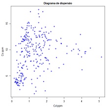
| 4.1 Scatterplot (download) | |
|
Plot a scatterplot of two quantitative variables. Variables to customize: varlistindex <- c(5,6) # index of the two GTD frame quantitative variablestitleGRAPH <- "Diagrama de dispersão" # title of the plottitleUNITS <- c("ppm","ppm") # units of the variables to add to axis legends |
 |
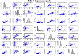
| 4.2 Scatterplot matrix (download) | |
|
Plot a matrix of scatterplots of several quantitative variables. Histograms are plotted in the diagonal of the matrix. Variables to customize: varlistindex <- c(5:11) # indexes of the several GTD frame quantitative variables |
 |
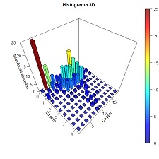
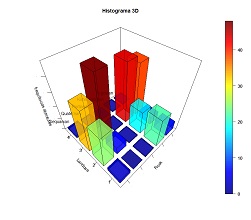
| 4.3 Contingency table and 3D histogram of two quantitative variables (download) | |
|
Compute a contingency table for equal size intervals of two quantitative variables (absolute frequencies) and plot a 3D histogram. Variables to customize: varlistindex <- c(5,6) # index of the two GTD frame quantitative variables |
 |
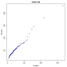
| 4.4 QQ plot (download) | |
|
Plot a QQ plot of two quantitative variables. Variables to customize: varlistindex <- c(8,10) # index of the two GTD frame quantitative variables |
 |
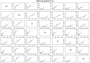
| 4.5 Matrix of QQ plots (download) | |
|
Plot a matrix of QQ plots of several quantitative variables. Variables to customize: varlistindex <- c(5:11) # indexes of the GTD frame quantitative variables |
 |
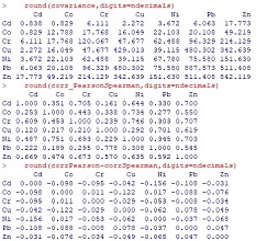
| 4.6 Matrices of covariance, Pearson and Spearman correlation and diferences (download) | |
|
For a set of quantitative variables, compute and display a matrix of covariance, a matrix of correlations (Pearson in the lower part and Spearman in the upper part) and a matrix of differences between Pearson and Spearman correlation coeficients. Variables to customize: varlistindex <- c(5:11) # indexes of the GTD frame quantitative variables |
 |
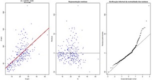
| 4.7 Simple linear regression (download) | |
|
Fit a linear regression (Y=aX+b) between two quantitative variables (left graphic) and display equation and R2, plot residuals vs the primary variable of the regression (central graphic) and plot residuals vs a normal distribution law (informal test for residuals normality). Variables to customize: varlistindex <- c(9,11) # index of the two GTD frame quantitative variables |
 |
| 4.8 Contingency table and 3D histogram of two qualitative variables (download) | |
|
Compute a contingency table for two qualitative variables (relative frequencies) and plot a 3D histogram. Variables to customize: varlistindex <- c(5,6) # index of the two GTD frame qualitative variables |
 |
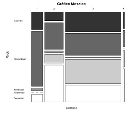
| 4.9 Mosaic diagram (download) | |
|
Plot a mosaic diagram of two qualitative variables. Variables to customize: varlistindex <- c(3,4) # index of the two GTD frame quantitative variables. Different order of the qualitative variables generate different graphics. |
 |
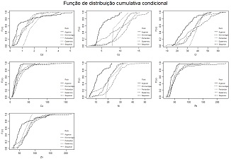
| 4.10 Conditional cumulative histograms (download) | |
|
Plot cumulative histograms of several quantitative variables conditional to the modalities of a qualitative variable. Variables to customize: varsepindex <- 4 # index of the qualitative GTD frame variable |
 |
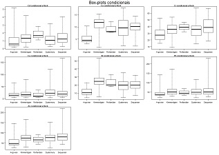
| 4.11 Conditional box-plots (download) | |
|
Plot box-plots of several quantitative variables conditional to the modalities of a qualitative variable. Variables to customize: varsepindex <- 4 # index of the qualitative GTD frame variable |
 |
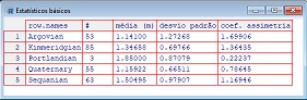
| 4.12 Conditional basic statistics (download) | |
|
Compute conditional basic statistics (mean, standard deviation and skewness) of a quantitative variable conditional to the modalities of a qualitative variable. Variables to customize: varsepvarindex <- 4 # index of the qualitative GTD frame variable |
 |