
7. Introduction to geostatistics and variograms
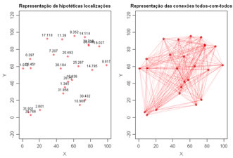
| 7.1 Link all pairs of points [Demo] (download) | |
|
Generate locations of a random dataset and connect all pairs of points. This demostrates the strategy behind the calculation of variograms, combine all pairs of points. Variables to customize: npoints <- 25 # number of locations to randomly generate |
 |
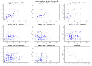
| 7.2 H-scatterplots (download) | |
|
Compute and display H-scatterplots, or self scatterplots of a unique variable measured at several locations. Each plot displays the values of the variable at a specific location and the values of the same variable at another location separared by a distance within and interval. For each plot a Pearson correlation coeficient is computed and at the end Correlation variations along distance (correlogram) is also plotted. Variables to customize: varcolXY <- c(1,2) # indexes of the coordinates X and Y in the GTD data frame |
 |
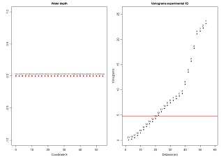
| 7.3 Experimental variograms 1D (download) | |
|
Compute experimental variograms for a list of values at 1D. Values are imported from an ASCII datafile. Left graphic display the location and the values. Right graphic represents the experimental variogram and the number of pairs of points of each value. Variables to customize: fileNameGrid="C:/temp/DemoGrid1d.prn"# name of the data file contains a list of values (grid 1D)fileNameMOD="C:/temp/Demogrid1D.MOD" # name of the output file for storing the experimental variogram to fit in scripts 7.10 and/or 7.11 |
 |
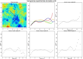
| 7.4 Experimental variograms 2D (grids) (download) | |
|
Compute experimental variograms for a list of values at 2D. Values are imported from an ASCII datafile, writted by Y and then by X. First graphic display the location and the values by colours, from blue to red. The second graphic represent all the 4 experimental variograms overlaped, and the remaining figures represent the experimental variograms one for each direction. Experimental variograms are computed and showed for four directions, N-S, E-W and diagonals. Variables to customize: fileNameGrid <- "C:/temp/Demogrid2D.out" # name of the data file contains a list of values (grid 2D) fileNameMOD <- "C:/temp/Demogrid2D.MOD" # name of the output file for storing the experimental variogram to fit in scripts 7.10 and/or 7.11 |
 |
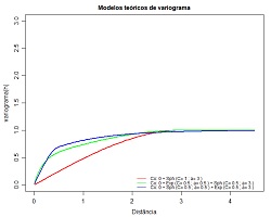
| 7.5 Plot theoretical models of variograms (download) | |
|
Plot several different theoretical models of variograms in the same plot for sake of comparison. Variables to customize: resolucao <- 200 # resolution of the representation (quality) maxmodels <- 10 # maximum number of functions to overlap (...) nmodels <- 3 # efective number of functions to overlap (... for each function ...) nugget_effect[1] <- 0.0 # nugget effect
nstructures_permodel[1]=1 # number of structures
model_type[1,1]="Sph" # theoretical function of the first structure (can be Sph, Exp, Gauss or Power)
model_type[1,2]="Sph" # theoretical function of the second structure (can be Sph, Exp, Gauss or Power)
sill[1,1]=1.0 # sill of the first structure
sill[1,2]=1.0 # sill of the second structure
range[1,1]=3.0 # range of the first structure
range[1,2]=3.0 # range of the second structure
(...)
cores <- c("red","green","blue","yellow","pink","black") # colours of each function |
 |
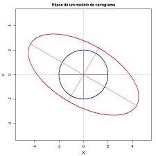
| 7.6 Plot theoretical ellipses of ranges (download) | |
|
Draw of ellipses showing several theoretical variograms structure ranges. Variables to customize: nstructures <- 2 # number of structures to represent
range <- c(2.0, 5.0) # major range of each structure
anisotropy <- c(1, 2) # anisotropy ratio for each structure
maindir <- c(0, 120) # angles of the main direction for each structure
maindir <- ifelse (maindir < 0, maindir+180, maindir) # do not change !!!
cor_elipse <- c("blue","red") # colours of each ellipse, one by structure |
 |
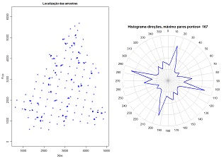
| 7.7 Azimuth angles histogram for 2D scattered data (download) | |
|
Compute azimuth angles for each pair of points and display a directional histogram. It is usefull for calculation of directional variograms in spatial scattered data. Variables to customize: varcolXY <- c(1,2) # indexes of the GTD frame X and Y coordinates passo <- 400 # interval of distance for azimuth calculations maxdist <- 400 # maximum distance for azimuth calculations (in this example calculations are made for pairs of points spaced by a distance between 0 and 400 meters sizePOINTS <- 1 # size of the points in the left plot ndecimals <- 3 # number of decimal places titleGRAPH <- "Localização das amostras" # title of the left plot |
 |
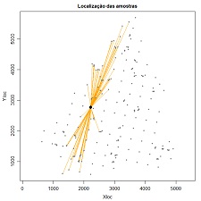
| 7.8 Demonstrate the selection of pairs of points for scattered data (download) | |
|
Plot lines conecting pairs of points at specific azimuth angles and tolerances and from a specific sample location. Variables to customize: sample <- 59 # one selected sample of the dataset varcolXY <- c(1,2) # indexes of the GTD frame X and Y coordinates anguloref <- 15 # azimuth angle for connection lines display angulotol <- 40 " tolerance angle for the azimuth angle ortogonaltol <- 500 # distance from the selected sample where the tolerance angle is not more applied titleGRAPH <- "Localização das amostras" # title of the plot |
 |
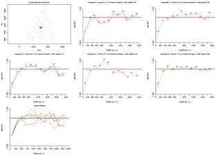
| 7.9 Experimental variograms for 2D scattered data (download) | |
|
Compute experimental variograms for a 2D scattered data set and save for the fitting step. The first plot show the location of the samples and the directions where the variograms are computed. Then, each plot show the experimental variogram of each direction. The number of pairs of points are displayed for each distance interval. At the end, a plot overlap all the experimental variograms. Each direction has a specific colour. Variables to customize: varcolXY <- c(1,2) # indexes of the GTD frame X and Y coordinates varlistindex <- 7 # index of the variable in the GTD frame fileNameOutMOD="C:/temp/CR.MOD" # name of the output file to store the experimental variograms unidadesdist <- "m" # units of distance plotLABELS <- TRUE # show or not the number of pairs of points in each plot padronizar <- TRUE # rescale calculations to one or not thresholdmax <- 1.00 # Percentile (max), to exclude samples thresholdmin <- 0.00 # Percentile (min), to exclude samples ndecimals <- 3 # number of decimal places
|
 |
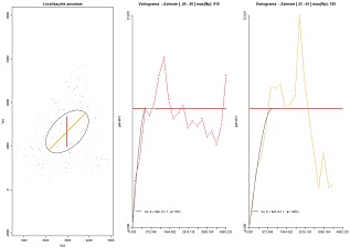
| 7.10 Fit theoretical models of variograms (fit for each direction) (download) | |
|
Fit theoretical models of variograms for each direction and represent the global ellipse and the ranges proposed for each direction for coherence purposes. Variables to customize: varcolXY <- c(1,2) # indexes of the GTD frame X and Y coordinates |
 |
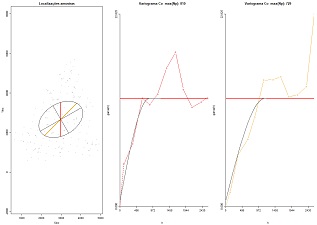
| 7.11 Fit theoretical models of variograms (fit ellipse) (download) | |
|
Fit theoretical models of variograms proposing the ranges of an ellipse. Variables to customize: varcolXY <- c(1,2) # indexes of the GTD frame X and Y coordinates unidadesdist="m"# units of distance
#
# Models are inputed by proportion of variance (sum of Nugget effect + Sills = 1)
#
nugget_effect <- 0.05 # nugget effect
nstructures <- 1 # number of structures
model_type <- c("Exp","Exp") # theoretical model of variogram
sill <- c(0.95,1.0) # sills of each structure
range <- c(1800,500) # major range
anisotropy <- c(1.5,1.0) # anisotropy ratios, ratio between major and minor ranges
maindir <- c(60,90) # azimuth angle of the main direction for each structure
maxX <- 2500 # maximum X distance |
 |